Formulas and Implementations from Scratch for Simple and Multiple Linear Regression

The formulas themselves are very short. As the first lesson in ESL, it’s very fundamental.

Many libraries can handle this, but I recently needed to compute regression using GPUs in development (which can accelerate calculations significantly). I thought I’d write a blog post to test if the website’s formula display works properly.

What is Linear Regression

Simply put, it’s using a linear equation to represent the trend in data.

Univariate: $y=mx+b$ Multivariate: $y=m_1x_1+m_2x_2+…+b$

You can imagine each point as a star of equal mass, and the regression line is like placing a long rod in this gravitational environment until it reaches its equilibrium position.

Simple Univariate Linear Regression Formula (Linear regression)

Simple OLS regression is listed separately because it’s more intuitive and easier to understand:

It’s simply the covariance divided by the variance of x. We’ll skip how to derive this formula, but you should already feel the elegance of it.

Then b can be obtained by plugging in m:

pyTorch Code Implementation

We use pyTorch for GPU acceleration. Let’s assume we have y as NVDA price data for February 2018:

import torch
y = torch.tensor([
    225.58, 228.8 , 217.52, 230.93, 228.03, 232.63, 241.42, 246.5 ,
    243.84, 249.08, 241.51, 242.15, 245.93, 246.58, 246.06, 242.  ,
    232.21, 236.54, 235.65, 242.16
])

Then we generate x:

x = torch.arange(len(y)).float()

tensor([ 0., 1., 2., 3., 4., 5., 6., 7., 8., 9., 10., 11., 12., 13., 14., 15., 16., 17., 18., 19.])

Regression code (here for readability, with some repeated calculations):

demean_x = x - x.mean()
demean_y = y - y.mean()
n_1 = x.shape[0] - 1
m = torch.sum(demean_x * demean_y / n_1) / torch.sum(demean_x ** 2 / n_1)
b = y.mean() - m * x.mean()
print(m, b)

(tensor(0.7734), tensor(230.4090))

Let’s plot to see the effect:

from matplotlib import pyplot as plt
plt.plot(x, y)
plt.plot(x, m * x + b)
plt.show()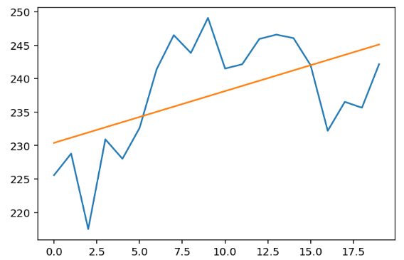

Looks good 🥂.

Multiple Linear Regression Formula (Multiple Linear regression)

The essence is the same as simple regression. Here we use matrix notation, which is even more concise:

A single formula solves everything, and it also applies to simple linear regression.

Side note, $X^TX$ appears everywhere, and there’s even a private equity firm named XTX.

pyTorch Code Implementation

The formula contains a lot of hidden information, and textual explanations are too cumbersome. Let’s implement it with code.

I’ve always thought that if textbooks and papers included corresponding code and step-by-step execution results for their formulas, there would be much less confusion when reading them, since making code executable requires complete information.

Here we demonstrate with bivariate linear regression. The most common example is using a quadratic equation ($y=ax^2+bx+c$), which is fitting a curve. Since it’s a univariate equation, why is it bivariate regression? Because the “bivariate” in regression refers to having 2 independent variables: $x, x^2$

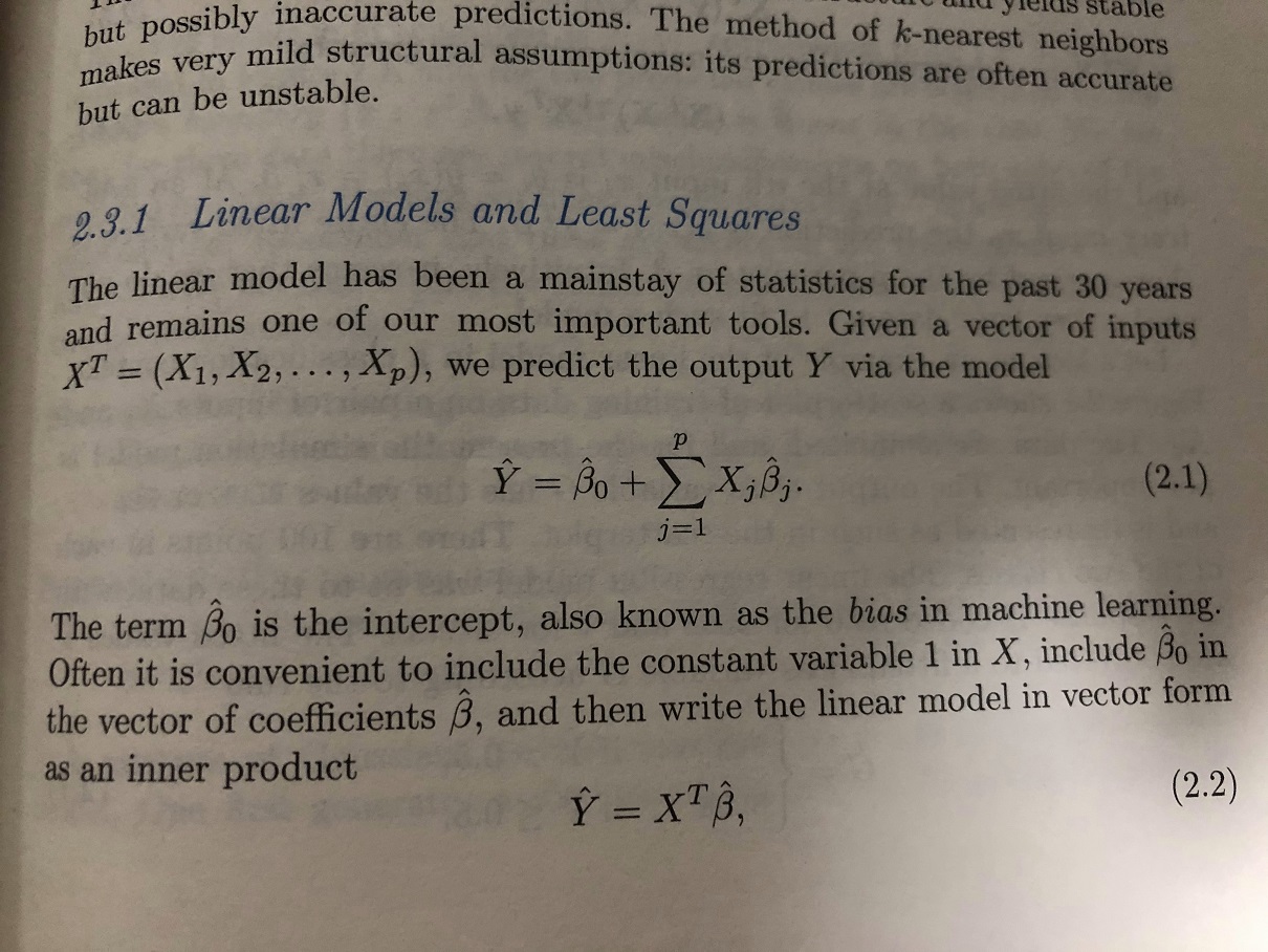
Still using the x, y data from above, first let’s generate the X matrix, containing $x, x^2$. Note that the first column here includes a constant 1 for matrix positive definiteness and to solve for b (shown as ${\hat\beta}_0$ in the figure):

X = torch.stack([torch.ones(x.shape), x, x ** 2]).T

tensor([[ 1., 0., 0.], [ 1., 1., 1.], [ 1., 2., 4.], [ 1., 3., 9.], [ 1., 4., 16.], [ 1., 5., 25.], … [ 1., 15., 225.], [ 1., 16., 256.], [ 1., 17., 289.], [ 1., 18., 324.], [ 1., 19., 361.]])

Then we can compute directly:

b, m1, m2 = (X.T @ X).inverse() @ X.T @ y
print(b, m1, m2)

(tensor(220.5210), tensor(4.0694), tensor(-0.1735))

Yes, this is the result. Let’s plot it:

plt.plot(x, y)
plt.plot(x, m1 * x + m2 * x**2 + b)
plt.show()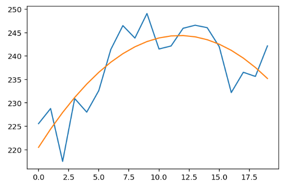

Perfect 👏. Is it simple? But actually, there are more important concepts later, such as multiple solution scenarios and orthogonal processing.

Collinearity and Orthogonality Issues

In practical use, problems solvable by simple polynomial regression are not common. Usually, regression is performed on observed values, and observed values are rarely completely independent, meaning the covariance between x’s is not zero. Keeping x’s independent ensures the coefficient is only responsible for that specific x and not influenced by other x’s, which requires orthogonal adjustment.

We won’t go into details here. If you want a quick solution, here’s a rough approach: use qr decomposition. After calculating with Q, R = torch.qr(X), use the formula $b, m_1,…,m_n=R^{-1}Q^Ty$ to solve.

If interested, you can refer to ESL 3.2.3 Multiple Regression from Simple Univariate Regression, which builds multiple regression from univariate regression.

Author: Zhang Jianhao Heerozh (heerozh.com)